Signal-to-Noise Ratio vs. Exposure
Having explored the components of noise in some detail, we are now in a position to condense our knowledge of Signal and Noise into a higher level of abstraction that we can use for camera selection. The information from the previous sections tells us about the two distinct imaging regimes – and we can now use SNR vs Exposure curves to model this behavior.
From the article titled Signal to Noise Ratio (SNR), we recall:
SNR = P*QE*t/ Sqrt(P*QE*t + Nr2 + Id*t) ——————– [Equation #3]
SNR vs Exposure and Relative SNR vs Exposure graphs are a convenient way to condense the previously shown information (Signal & noise sources vs. Exposure) into a single curve for a particular imaging setup.
All four of the following graphs represent the same imaging scenario: the performance of our test imager [QE=80%, Nr=2e- and Id = 0.47e-/p/s @ -5°C] with a Photon Flux of 25 Photons/pixel/sec. The performance is shown in four different ways: (1) Signal and noise vs Exposure, showing the Read Noise limited and Photon Shot Noise limited regimes (2) SNR vs Exposure (3) SNR vs Exposure, with Ideal Imager for comparison (4) Relative SNR vs Exposure, in which SNR has been normalized relative to the SNR of an Ideal Imager. Note that Dark Shot Noise is negligibly small in this example.
From details of Noise Sources …
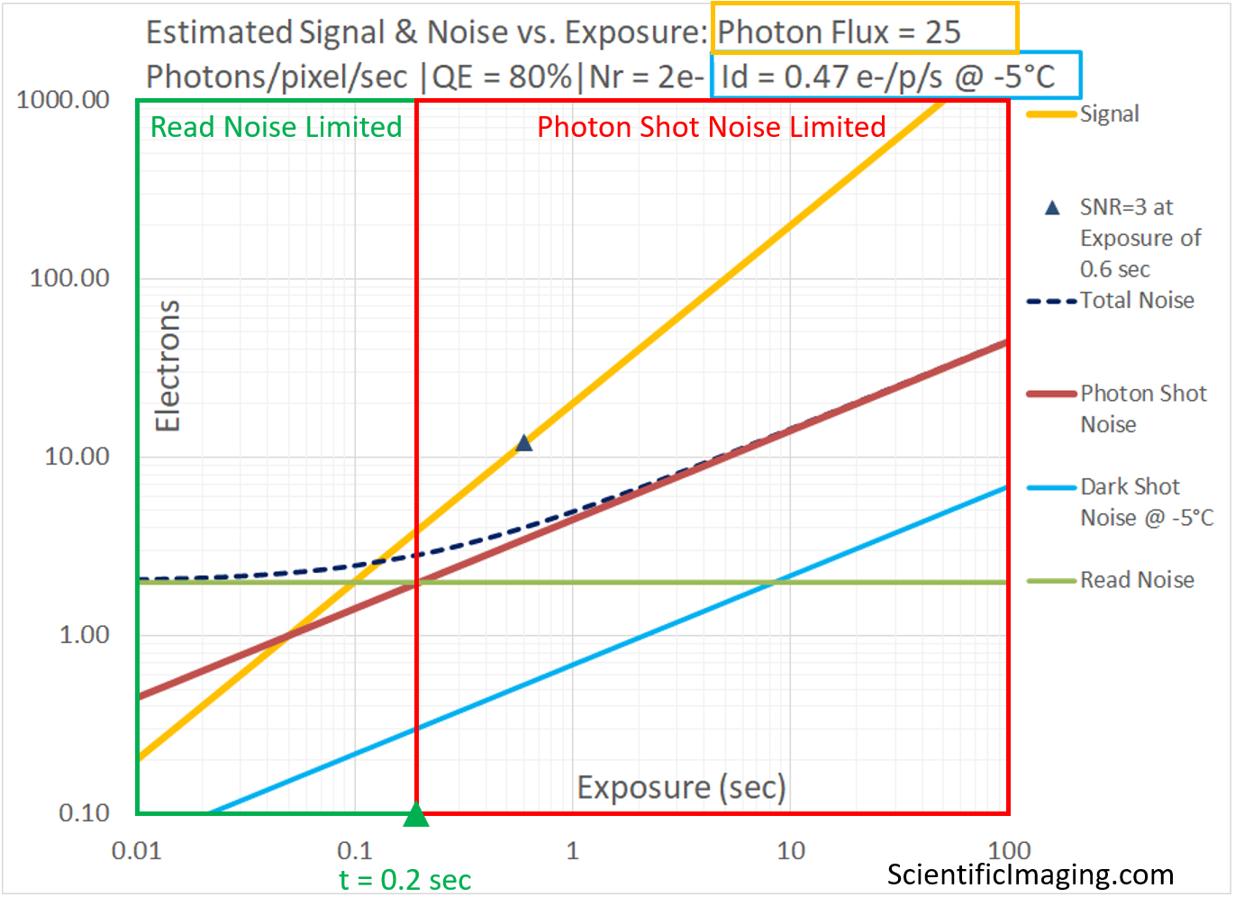
… to a single SNR vs. Exposure curve
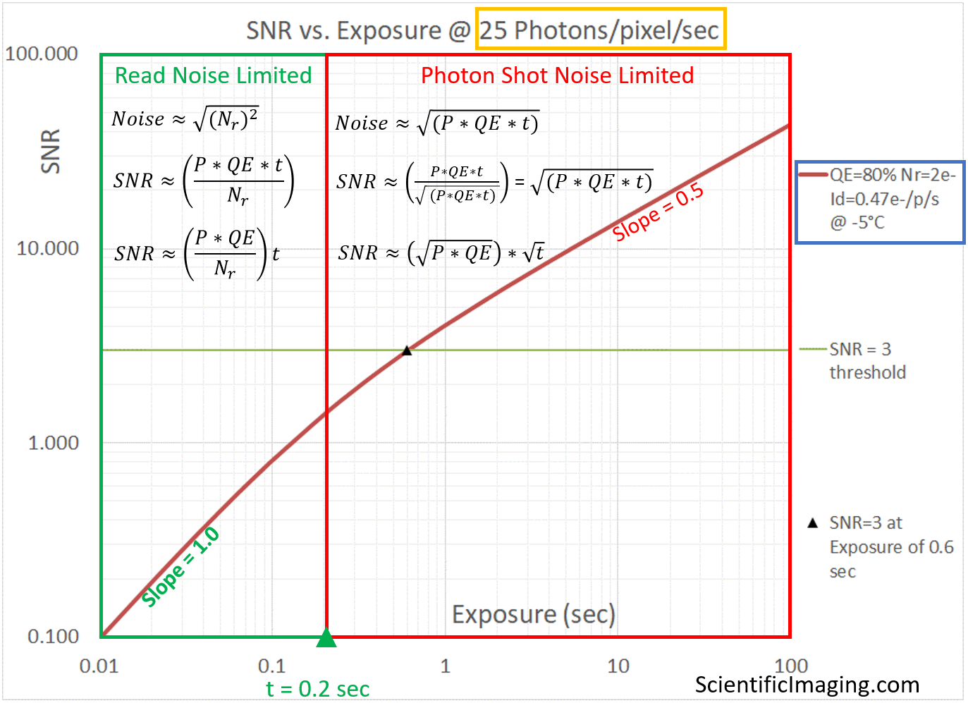
The two noise-limited regimes are characterized by the equations shown above, with appropriate assumptions and simplifications applied (as described earlier in the article titled Noise-limited Performance of Cameras).
The equations shown in the graph tell us that SNR has a linear relationship with exposure in the Read Noise limited region and a square-root relationship with exposure in the Photon Shot Noise limited region. This means that a doubling of exposure will provide a 2x improvement in SNR in the Read Noise limited region, but only a Sqrt(2) improvement in SNR in the Photon Shot Noise limited region.
It is for this reason that one should – in general – seek the longest exposure that the sample and the imaging workflow can sustain. As long as the system is Read Noise limited, a 2x increase in exposure will result in a 2x improvement in SNR. But once past the “knee” of the above curve, the system is Photon Shot Noise limited and it will take a 4x change in exposure to gain an additional 2x improvement in SNR.
The insight that SNR has a linear relationship with exposure in the Read Noise limited region also helps us answer a question that comes up frequently in low-light applications:
Question: is it better to average several exposures, or to take a single long exposure.
The short answer: it depends on whether the system is Read Noise limited, or Photon Shot Noise limited. In a Read Noise limited system, a single long exposure will provide an image with a higher SNR. In a Photon Shot Noise limited system, both techniques achieve the same SNR – temporal averaging can be advantageous when considering artifacts such as “hot pixels”, which are much more of a problem at long exposures. Details follow.
A) consider a system that is Read Noise limited for exposures up to 1sec. The same number of photons are collected if we take 10 images at an exposure of 0.1sec as when we take one image at an exposure of 1sec. Since SNR has a linear relationship with exposure in a Read Noise limited system, the single image taken with an exposure of 1sec has an SNR that is 10x the SNR of an image taken at an exposure of 0.1sec. Since uncorrelated noise adds in quadrature, averaging the 10 images that were taken at an exposure of 0.1sec will increase the SNR by the square root of the number of exposures. In our example, the resulting SNR of the averaged image is a factor of Sqrt(10) i.e. ~3x the SNR of an image taken at an exposure of 0.1sec. Therefore, we can say that the image taken at an exposure of 1sec will be Sqrt(10) or roughly 3x higher SNR than an image that is captured by temporally averaging 10 images that were taken at 0.1sec. Therefore, for Read Noise limited imaging: all else being equal, it is better to take a single exposure at a longer exposure than to do temporal averaging of images taken at shorter exposures.
B) in a system that is Photon Shot Noise limited, the SNR is proportional to the Sqrt of the exposure – it is NOT a linear relationship, as in the case of a Read Noise limited system. Extending the example considered in (A), we examine the difference between ten exposures of 10-seconds duration and a single 100-second exposure, both of which acquire the same number of photons. The image taken with an exposure of 100sec has an SNR that is only Sqrt(10) i.e. ~3x better than the images taken with an exposure of 10sec. Temporal averaging of the 10 images taken at exposures of 10sec would provide an improvement of Sqrt(10) i.e. ~3x. Both methods achieve the same SNR. Therefore, in a Photon Shot Noise limited system, temporal frame averaging and long exposures provide images with the same SNR, all else being equal.
Note: there may be other considerations that make temporal averaging a useful technique in Photon Shot Noise limited systems. For example, a long exposure of 100sec is likely to result in more “hot pixels” than a temporally averaged series of images taken at exposures of 10sec.
Hot pixels: due to impurities and imperfections in the manufacturing process, some pixels can have a higher dark current than others. Depending upon the manufacturer, the dark current for these “hot pixels” can be several multiples of the nominal dark current specification for an imager. This is not an issue at short exposures, but at longer exposures, hot pixels can show up as bright points in the image, giving the appearance of a star field when a dark image is taken at a long exposure. Since dark current doubles for every 6-7 degrees C rise in temperature, the effect is even more pronounced at higher temperatures. Cooling the image sensor reduces the dark current for all pixels, including the fraction of pixels that are “hot”. Cooling thus mitigates the effect of hot pixels, making them less visible, although the use of numerical enhancement post-processing of images can make this artifact visible.
Since the above graph captures the essence of the camera’s performance under the given conditions, it can be used as the basis to compare the performance of a camera under two different imaging conditions, or between two different cameras under the same imaging conditions. As we will see shortly, it is useful to show multiple scenarios on one graph and make decisions with respect to camera selection.
Comparing real-world imagers with an Ideal imager
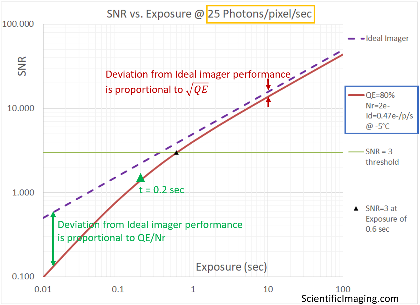
Since the SNR vs. Exposure plot can show multiple cameras, let us begin by using it to compare the performance of an Ideal camera with a real-world camera in which Photon Shot Noise and Read Shot Noise are the only sources of temporal noise – in other words, we assume that Dark Shot Noise is negligibly small.
Note that the Ideal imager is only limited by Photon Shot Noise. For this reason, there aren’t two distinct imaging regimes shown on the above graph.. The real-world camera does exhibit two distinct noise-limited regimes, and can be shown to deviate from Ideal camera behavior in two different ways with a crossover at exposure t=0.2 sec, shown by the green marker. The lower-left region of the graph (which represents the Read Noise limited behavior of the camera), curves away from the Ideal camera behavior by an amount that is proportional to QE/Nr. Towards the top RHS of the graph, the line representing the camera deviates from Ideal camera behavior by an amount that is proportional to the Sqrt(QE).
This indicates that (at least) two different figures-of-merit are relevant in the two regimes.
It also tells us that if our imaging conditions are such that the system is Photon Shot Noise dependent, i.e. the system is not extremely light-starved, then one does not need to specify cameras with the lowest Read Noise specifications. One may obtain high SNR images with CMOS cameras, and cameras may be selected based on other parameters such as Field-of-View, frame rate and cost. While a higher Quantum Efficiency is always a plus, one can often use a camera with slightly less QE and compensate by increasing the exposure setting. This is a tradeoff that is usually acceptable because exposure-durations that are less than the readout time of an imager do not necessarily impact the overall frame rate in a typically overlapped exposure-readout sequence.
On the other hand, if our system is light starved, it is likely to be Read Noise limited and a camera with a high QE AND a low Read Noise will be very beneficial. sCMOS cameras are well suited for these conditions. In such cases longer exposures are also beneficial, since SNR has a linear relationship with exposure until the crossover point . Beyond the crossover point, the system becomes Photon Shot Noise limited, and SNR is proportional to the Sqrt of exposure, requiring, for example a 4x increase in exposure for a 2x improvement in SNR.
Relative SNR makes comparisons easier
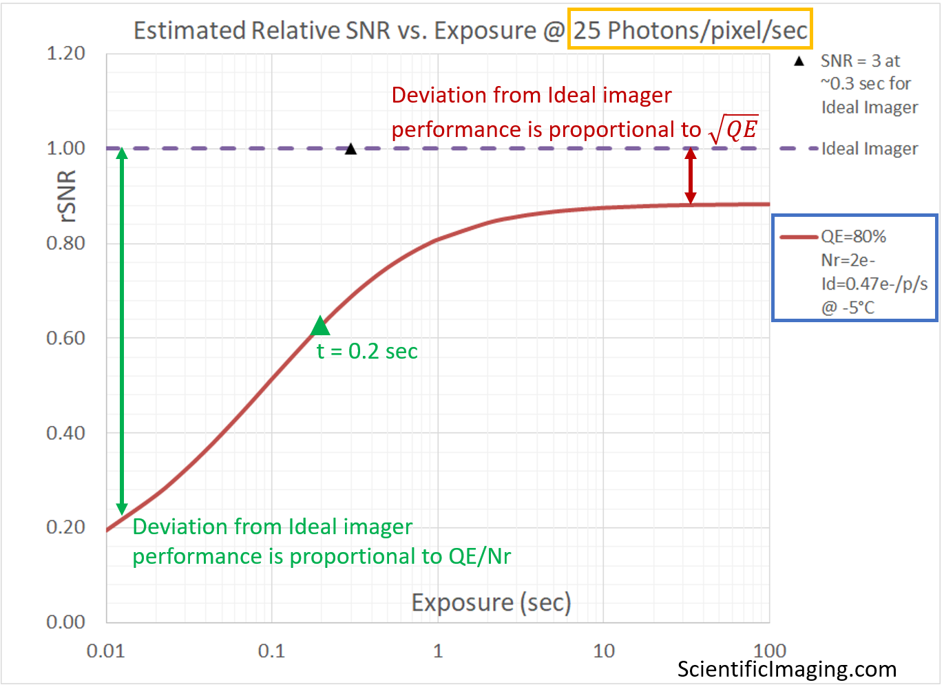
As in the case of the SNR vs. Exposure graph, it is convenient to show multiple cameras on a Relative SNR graph to make comparisons, leading to purchasing decisions. Since the Ideal camera sets the theoretical maximum for the achievable SNR, it is useful to see how different cameras deviate from the theoretical maximum, under a certain set of conditions. This graph is also useful because it amplifies the difference, particularly towards the Read Noise limited end. This makes it possible to observe relatively small differences between cameras which would likely be obscured on an SNR vs Exposure graph. Note that the deviation from Ideal camera behavior on the lower-LHS side (the Read Noise limited region) is a function of QE and Nr, while the deviation from Ideal behavior on the top RHS end (the Photon Shot Noise limited region) is a function of the QE.
As in the previous case, the assumption is that Dark Shot Noise is negligibly small.
Real-world imagers
We are now in a position to apply the above methods to real-world cameras. In the following section, we compare three different classes of cameras by means of SNR vs Exposure and Relative SNR vs Exposure graphs:
- TE-cooled sCMOS cameras: e.g. Dhyana 95 V2, pco.edge 4.2bi
- non-cooled sCMOS cameras: e.g. pco.panda 4.2bi
- non-cooled CMOS cameras: e.g. Sony Global Shutter Pregius cameras (Gen 2 and Gen3)
The goal of this section is to show the strengths (and one major weakness) of this method. It is a convenient way to compare several cameras under a similar range of imaging conditions. In this case we run the model for two different levels of Photon Flux. We select 90 photons/pixel/sec to represent the higher end of “low-light” conditions for which an Ideal imager would be able to achieve an SNR=3 at an exposure of 0.1sec. For this level of Photon Flux we can use our model to estimate the SNR of various cameras over a range of exposures [from 0.01s or 10ms to 100sec]. A similar analysis is performed for a Photon Flux of 9 photons/pixel/sec to represent the lower end of “low-light” conditions for which an Ideal imager would be able to achieve an SNR=3 at an exposure of 1sec.
Note that the Relative SNR vs. Exposure plot on the RHS represents the same conditions, with the value of SNR normalized to that of an Ideal imager (as in previous sections). The Relative SNR plot gives us an amplified view of the smaller differences between different cameras that may be more difficult to discern in the SNR vs Exposure plot.
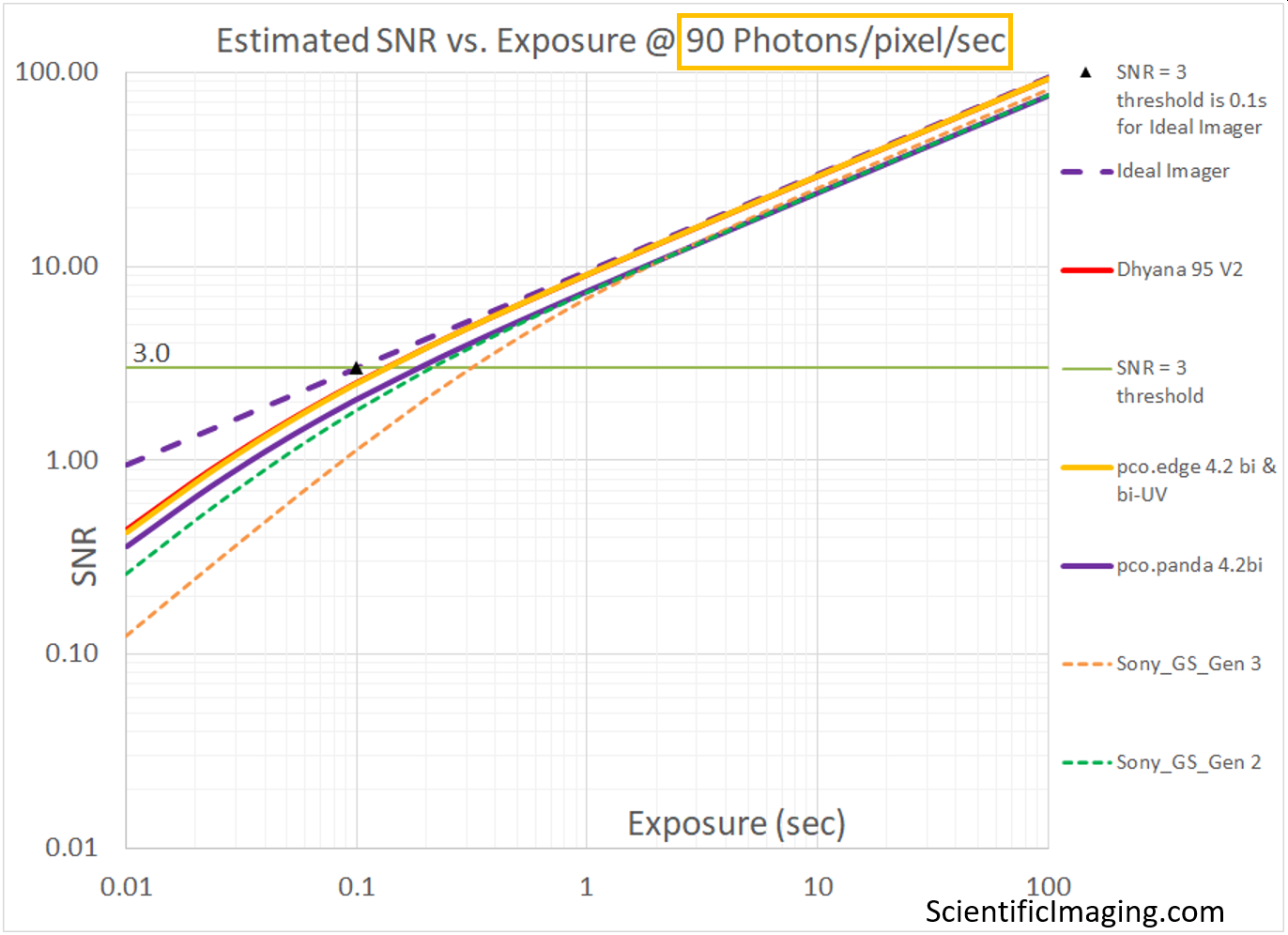
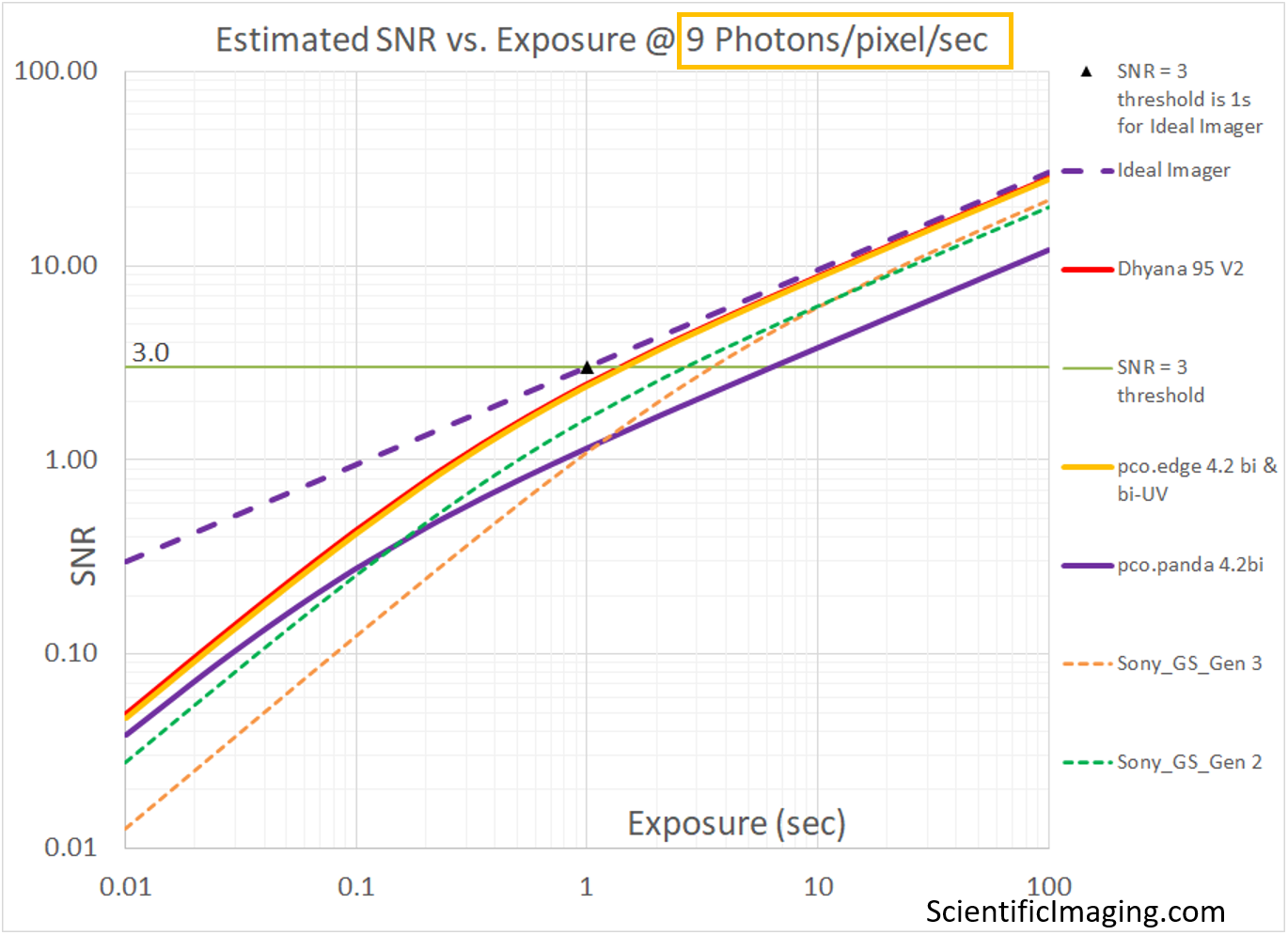
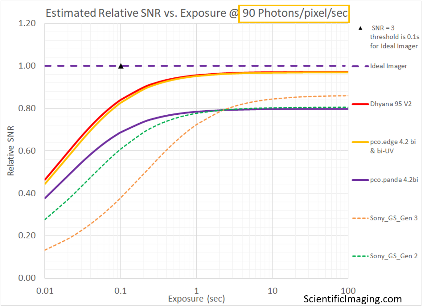
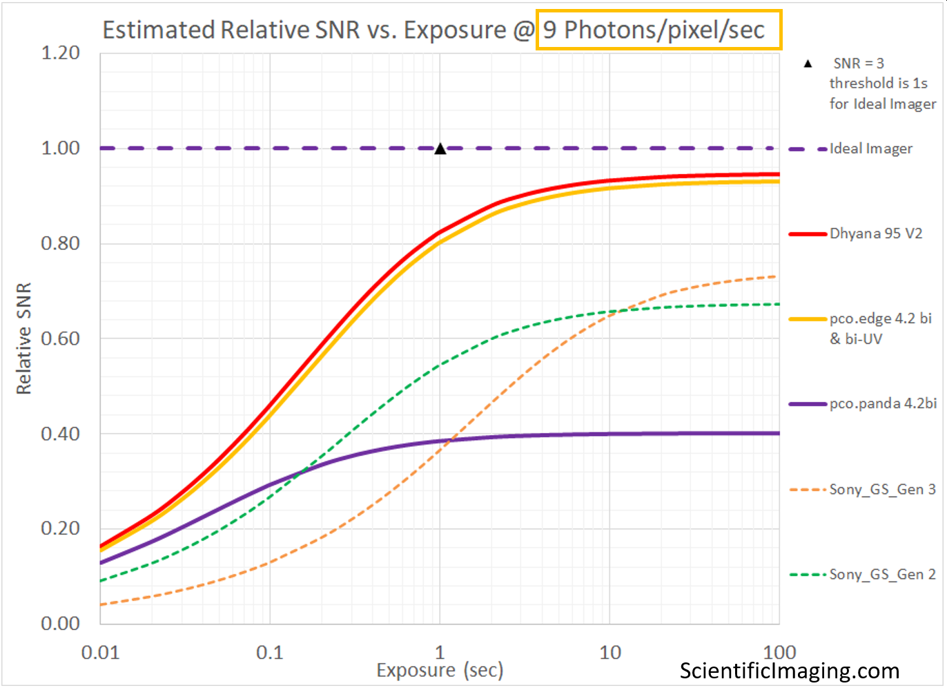
The weakness of the method is that it does not account for the size of the pixels in different cameras. When this detail is obscured by our choice of units (as Photons/pixel/sec), a cooled sCMOS camera with 11um pixels appears to achieve the same SNR as that of a cooled sCMOS camera with 6.5um pixels. Non-cooled CMOS cameras with 4.5um and 3.45um pixels appear to outperform non-cooled sCMOS cameras with 6.5um pixels. This weakness is addressed in the next section.
Taking Pixel Size into account
Until now, we have not taken Pixel Size into account, by simply choosing our independent variable as Photon Flux (units: Photons/pixel/second) and not Photon Flux Density (units: Photons/sq-μm/second). The implicit assumption behind this choice is that the same number of photons/sec are incident on a small pixel with an area of, for example, 2.5μm x 2.5μm as on a larger pixel with an area of 6.5μm x 6.5μm. For this to be true, the optical magnification of an imaging system must change such that both pixel sizes represent the same area in the sample plane. While this is certainly possible, it doesn’t represent a typical comparison between cameras in which one camera is simply replaced by another with no change in the optics. To properly model such a comparison, it is better to assume that the Photon Flux Density (units: Photons/sq-μm/second) is the same between the A and the B cameras.
Note: the size of the pixels in a camera also impact the optical resolution of the imaging system. In the context of SNR, increasing the size of a pixel may improve the SNR (all else being equal), but its effect on optical resolution must also be taken into account. This is covered in some detail in Knowledge Base articles titled How diffraction limits the optical resolution of a microscope and Optical Resolution of a Camera and Lens system.
The condition of having the same Photon Flux Density on different cameras may be simulated by making a small change to our method – using Photon Flux Density (units: Photons/sq-μm/second) as the independent variable “P”. Our equations must change slightly: essentially we are replacing “P” with “P*a”, where “a” represents the area of the pixel in sq-μm. In this manner, we incorporate pixel area into both Signal and Noise and thus SNR.
S (in electrons) = P *a*QE*t ———————– [Equation #4]
Noise = Sqrt(P*a*QE*t + Nr2 + Id*t) ——————— [Equation #5]
SNR = P*a*QE*t/ Sqrt(P*a*QE*t + Nr2 + Id*t) ——————– [Equation #6]
In the above equation: P = Photon Flux Density (units: Photons/sq-μm/second); a = pixel area in sq-μm. Since an Ideal imager is one that has infinitesimally small pixel, we can’t really compare real-world imagers with an Ideal imager in this framework. But we can very efficiently compare different real-world imagers on one graph (SNR or rSNR).
The sequence below shows the importance of factoring in the area of the pixel into our SNR and Relative SNR vs Exposure analyses. The Photon Flux Density values of 7.6 and 0.76 Photons/sq-μm/sec are chosen to represent the same Photon Flux of 90 and 9 Photons/pixel/sec as in the above example, on a pixel of 3.45μm x 3.45μm. This is the pixel size for Sony’s Pregius Global Shutter Gen2 imagers, which have a pixel area of 3.45 x 3.45 = 11.9sq-μm. 90 Photons/pixel/sec is equivalent to 90/11.9 = 7.6 Photons/sq-μm/sec and 9 Photons/pixel/sec is equivalent to 9/11.9 = 0.76 Photons/sq-μm/sec – hence the choice of those values for Photon Flux Density in the comparison below. Due to this selection of values, the line representing the Sony_GS_Gen 2 imagers in the SNR vs. Exposure graph is the same as that in the above sequence.
In the analysis shown below, the number of Photons/pixel/sec scale with the pixel area of each imager and one can see the estimated performance of the different imagers is quite different from that of the previous analysis that did not account for pixel size. This method provides information that is more representative of the situation in which cameras are swapped in and out without changing the optical magnification.
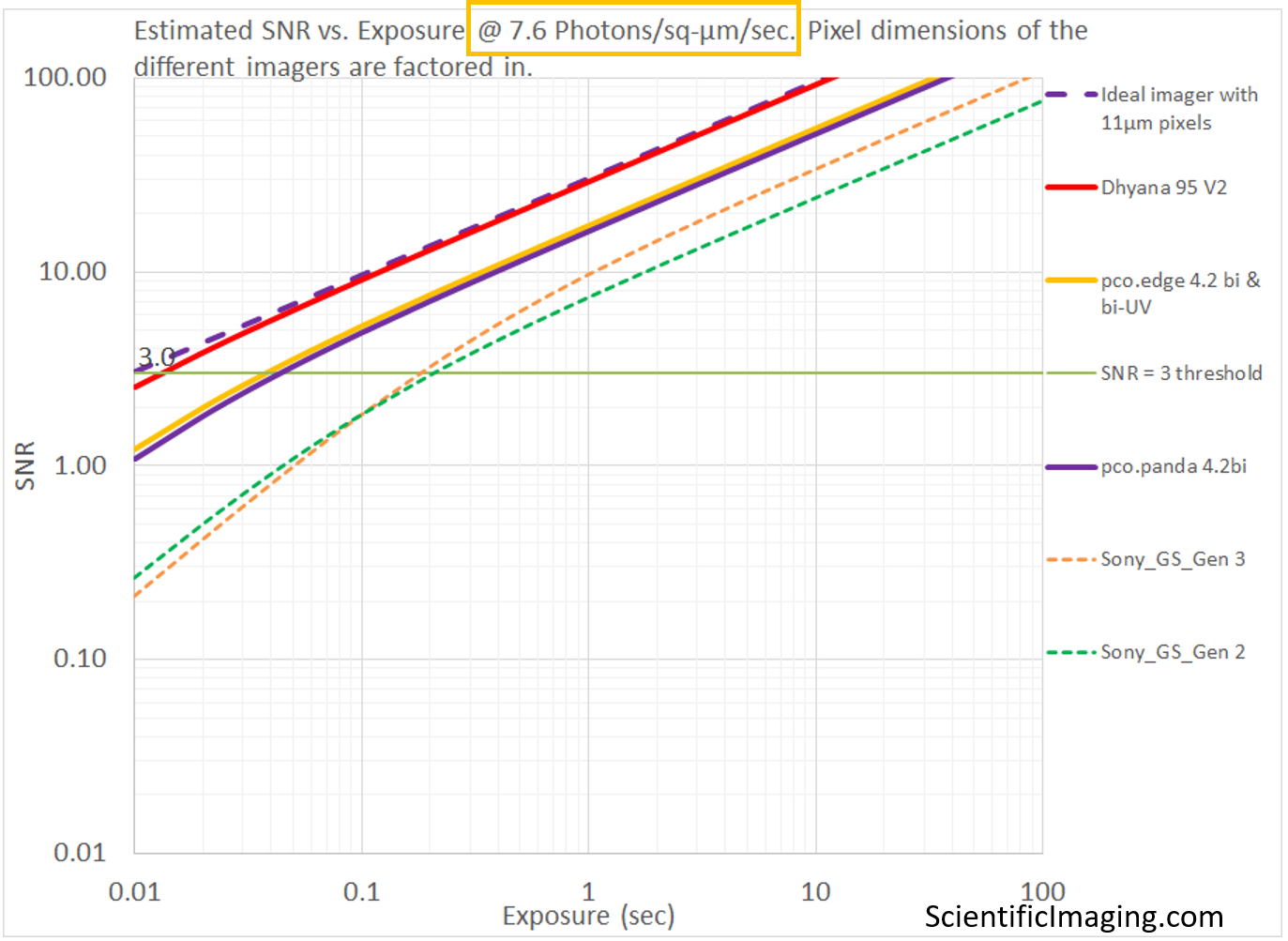
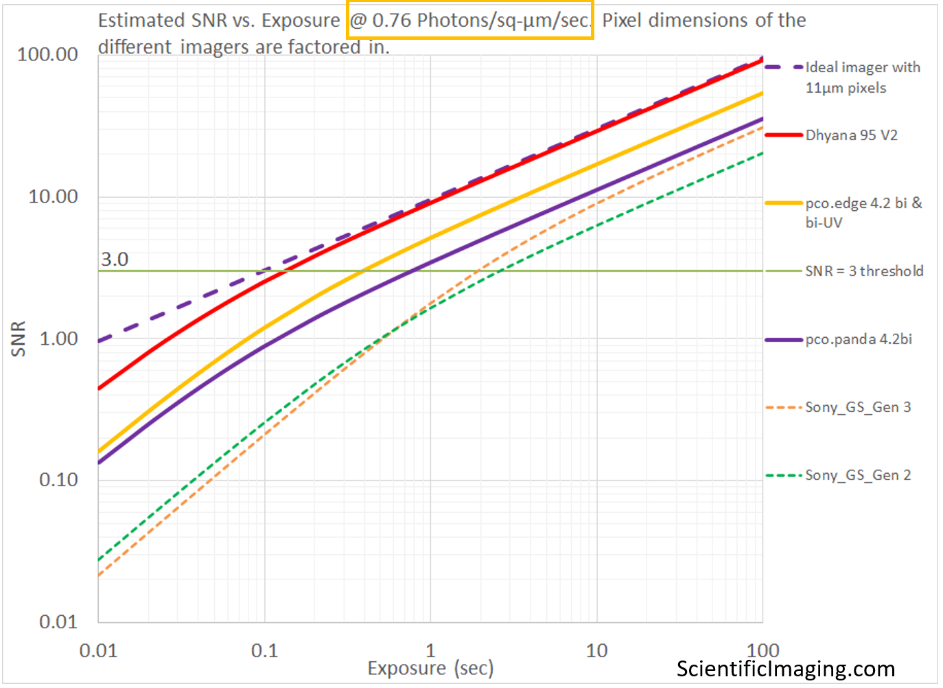
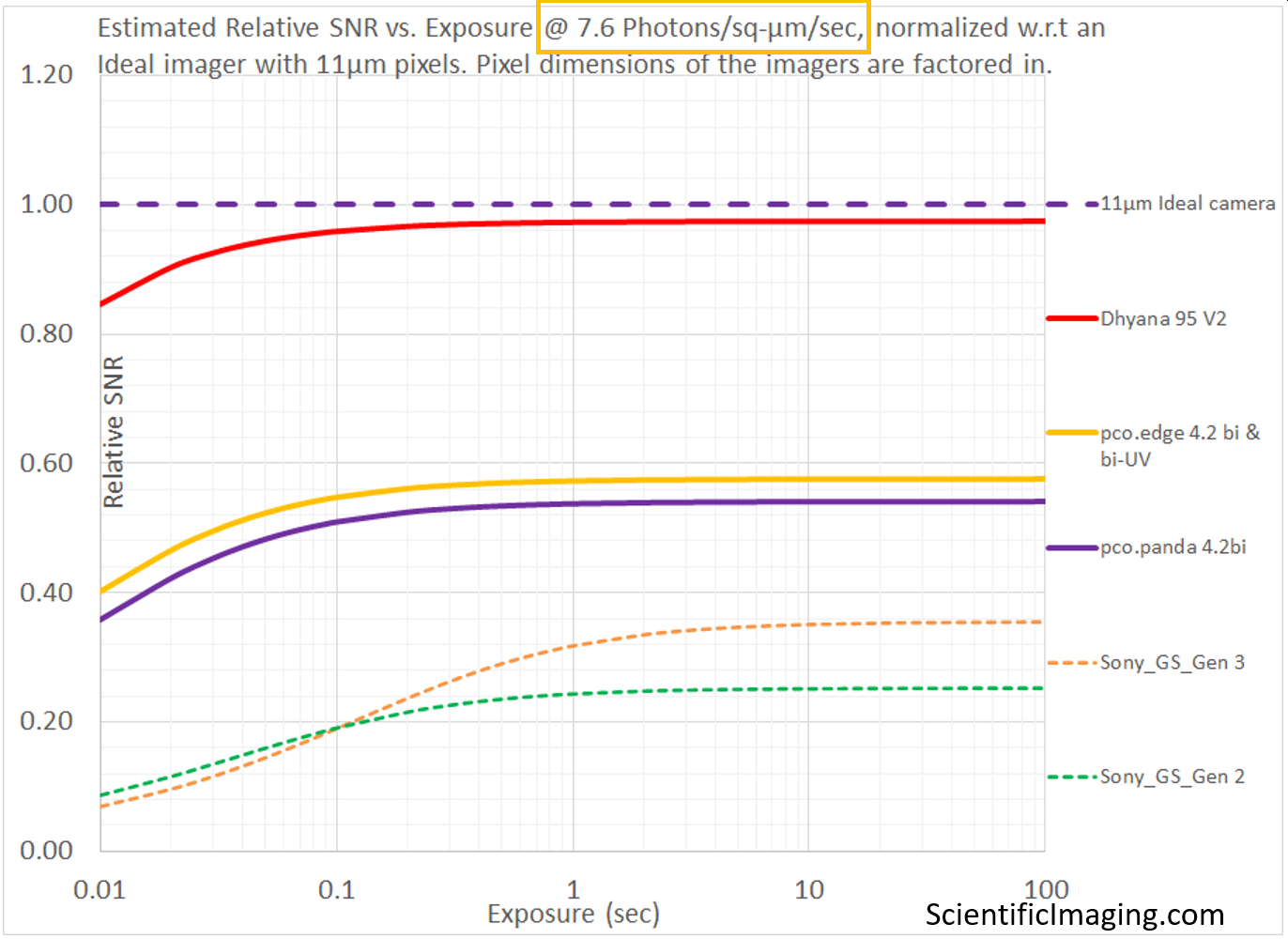
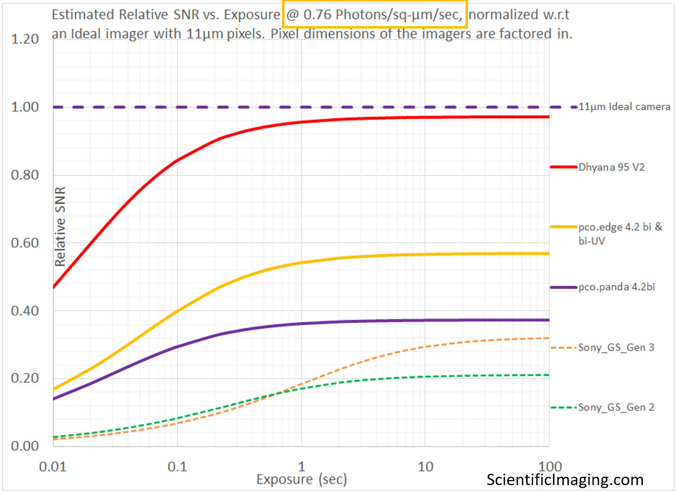
Since there isn’t a proper way to model an Ideal imager with infinitesimally small pixels, one can use any imager of a certain pixel size as the reference in the Relative SNR vs. Exposure graph. In the example above, we have normalized the rSNR (Relative SNR vs Exposure) values based on a “somewhat ideal” imager with 11μm pixels with no Read Noise and no Dark Current.
When seeking to replace an older or obsolete camera in an imaging system, it is often convenient to use the performance specifications of the older camera as the reference for the purposes of normalization. In this manner, several prospective cameras can be benchmarked against a known reference during the selection process.
In the next article, we wrap up the discussion on benchmarking cameras by means of various figures-of-merit.

